A maximally tiny language model
What can a 552-parameter language model do?
In this post I document a little experiment I have been playing around with for a while that explores an absolutely minimal language model. I’m specifically interested in how small a language model can be made while still doing something. I got the idea while I was reading a post about GPT-2. A pre-COVID model, GPT-2 now seems minuscule in comparison to current frontier models. Its largest incarnation was trained on about 40 GB of text, had 1.5B parameters and used an embedding dimension of 1600. Nowadays, a GPT-2-like model can easily be trained in a consumer GPU with ~16-24 GB of VRAM.
If the GPT-2 family of models pales in comparison to current model dimensions, the model I present here today pales in comparison to GPT-2. Since it is extremely minimal, it can be trained on a single CPU core in a few seconds and needs very little RAM. It can have single-digit embedding dimensions, does not follow the transformer architecture, has no attention mechanism, and may not even use any hidden layers! It is a purely academic model, in the sense that it is absolutely simple but does nothing useful.
I’ll call the language model in this post TinyLM. Below is a summary of some of the features and concepts that this post touches on:
- A closed world. 92 words, a few hard rules, 2560 sentences. That is all the language there is.
- Learned embeddings. Nobody tells the model that “wine” and “beer” belong together. It works it out from the sentences alone.
- A bag of words. Words go in unordered, so “the chef met the clerk” and “the clerk met the chef” look exactly the same to the model.
- A ceiling of about 48.4%. Throwing the order away caps accuracy, no matter how big the model gets.
- A few hundred to a few thousand parameters, with the embedding size and the hidden layer size as free knobs.
- A sweep over those two knobs, from the baseline all the way up to the ceiling.
Since it is so easy to train and test, the model is fluid. It can have between a few hundred and a few thousand parameters, depending on the dimensionality of the embeddings and the size of the hidden layer. But let’s start at the beginning.
The world
Such a small model wouldn’t fare very well trying to reproduce human language, so I reduced it to a set of predefined sentences. I call this set our closed world. This world is composed of only 92 words: 8 proper names, 12 actors, 6 prepositions, 28 places, one determiner, 24 objects, and 13 verbs. Everything that can be expressed is done through those 92 words. I combined them using some rules and got the 2560 possible sentences that constitute our world. This is the whole world. This is the training dataset. This is everything TinyLM will ever be able to learn and recognize.
Every sentence in the world has the same shape: a subject, a verb, an object, and sometimes a place. Subjects are always people. There are 20 of them, either a bare name (“john”, “mary”, “lucia”) or “the” plus an occupation (“the chef”, “the pilot”, “the farmer”). The verbs come in two families. Four of them (“helped”, “met”, “thanked”, “invited”) are things you do to a person, so the object is another person and never the subject itself: “lucia invited mary” is in the world, “lucia invited lucia” is not. The other nine are things you do to stuff, and each one only takes objects of the right kind. You drink drinks, you eat food, you repair tools and homeware, you pack clothes and drinks. So “the chef ate soup” exists, “the farmer repaired the soup” does not.
Finally, about half of the sentences end with a place: “near the bridge”, “inside the cellar”, “under the tower”. That’s the whole grammar. No questions, no negation, no conjunctions, no subordinate clauses, no adjectives. Just subject, verb, object, and sometimes where.
A few real sentences out of the 2560, so you can see the shape:
the pilot met john near the cellar– person verb, subject and object both people, place at the end.lucia invited mary– the same, without the place.john drank wine behind the hut– thing verb, and the object is a drink because “drank” only takes drinks.the clerk organized books under the store– thing verb, object from the paper class.- And two that are not in the world:
lucia invited lucia, because you cannot invite yourself, andthe farmer repaired the soup, because soup is not a tool.
Model structure
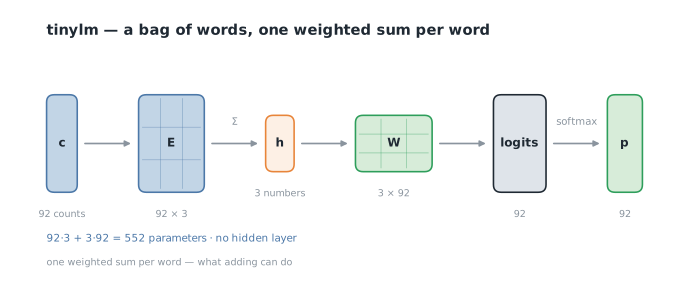
The whole model is two small tables of numbers. The first one gives every word a handful of coordinates: three numbers per word in the default model, so \(92 \times 3 = 276\). The second one, the readout, says how much each word likes each of those three directions, another 276. That’s it, 552 numbers in total. There is no lookup table of sentences and no rules inside, just those numbers. All of them are learned from the world above.
The pipeline for guessing a word is almost embarrassingly simple:
The architecture
92 counters go in, the \(92 \times 3\) coordinate table turns them into 3 numbers, the readout scores all 92 words, and softmax turns the scores into percentages. That is the whole default model: 552 numbers and no hidden layer.
The same three steps, written as matrix operations. Count the words of the sentence into a vector \(\mathbf{c}\) with one entry per word in the world, and let \(\mathbf{E}\) be the table of coordinates, 92 rows of 3 numbers. The sentence collapses into a single point by adding the rows of the words that appear, the readout \(\mathbf{W}\) scores that point against every word, and a softmax turns the scores into percentages:
$$ \mathbf{h} = \mathbf{c}^{\top} \mathbf{E} \qquad \mathbf{z} = \mathbf{W} \mathbf{h} \qquad \mathbf{p} = \operatorname{softmax}(\mathbf{z}) $$
with \(\mathbf{E} \in \mathbb{R}^{92 \times 3}\) and \(\mathbf{W} \in \mathbb{R}^{3 \times 92}\), so \(\mathbf{h}\) is a column of three numbers, \(\mathbf{z}\) (logits) is a column of 92 scores and \(\mathbf{p}\) is the column of 92 probabilities that this post keeps calling percentages. Each row of \(\mathbf{W}\) belongs to one word and says how much that word likes each of the three directions, which is the readout table above read along the other axis. The code keeps it transposed, as a \(3 \times 92\), which changes nothing except the order of the indices.
The model in one picture
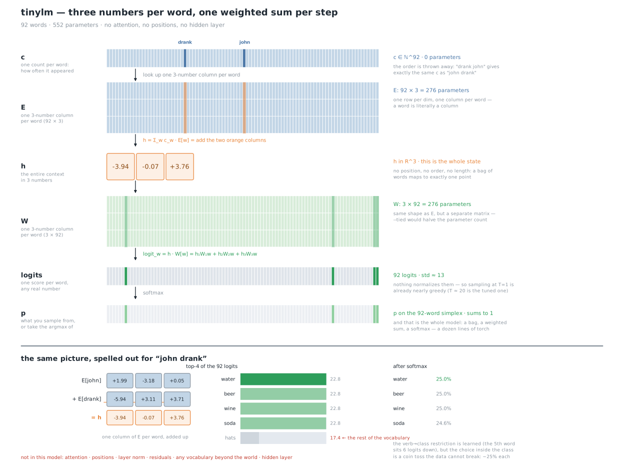
The whole thing with real numbers for “john drank”. A row of 92 counters, the (92 times 3) table of coordinates, the two rows that matter added into one point, the readout scoring all 92 words, and the softmax at the end. The bottom half adds up the coordinates of “john” and “drank” by hand and shows why the four drinks end up within a tenth of a point of each other.
The middle step is worth a second look. The sentence is turned into a row of 92 counters, one per word, saying how many times each appears. Two words show up, so two counters are 1 and the other ninety are 0. Looking up the coordinates of each present word and adding them gives a single point, and that point is the model’s entire idea of what the sentence is about so far. Then each of the 92 words gets a score for how well it lines up with that point, and the highest score wins. Three multiplications and two additions per candidate word, and that is the whole network.
This is where the “bag of words” in the summary comes from. The input is a bag of counters, and counting does not care about order. Adding numbers does not care either: 3 + 5 is the same as 5 + 3. So “the teacher drank” and “the drank teacher” land on exactly the same point, get exactly the same scores, and the model happily finishes the nonsense one.
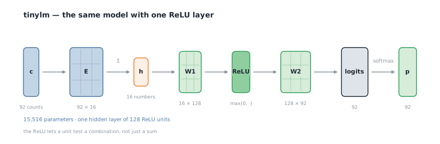
The optional hidden layer is the one part that is not just adding. It sits between the point and the scores and turns the single “how well does this word line up” question into a set of small yes/no questions about the context, something like “was john seen?” and “was cleaned seen?”. Because each of those answers can be silent when it does not apply, the model can score a word high only when both conditions hold, which plain adding cannot express. In symbols, the readout becomes
$$ \mathbf{z} = \mathbf{W}_2 \operatorname{ReLU}(\mathbf{W}_1 \mathbf{h} + \mathbf{b}_1) + \mathbf{b}_2 $$
The same picture with one ReLU layer
The same model with 16 numbers per word and a hidden layer of 128 units: the point becomes 16 numbers, W1 turns it into 128, the ReLU keeps the positive ones, W2 scores the 92 words, and softmax does the rest. 15516 numbers in total, and this is the version that reaches the ceiling.
with \(\mathbf{W}_1\) of size \(3 \times k\) and \(\mathbf{W}_2\) of size \(k \times 92\), plus one bias per hidden unit and one per word. A narrower point also limits how much the hidden layer can help, which is why the interesting knob turns out to be the number of coordinates per word rather than the size of the hidden layer. As we’ll see shortly, at 16 coordinates per word and 128 hidden units the model has 15516 parameters and reaches the ceiling. The default is still the 552-number version (because the point of the experiment is the smallest thing that works!).
Accuracy ceiling
Nobody can score 100% here, and the reason is that the world is non-deterministic by design. After “john drank” any of the four drinks fits, and nothing in the sentence says which one you meant. On average a bag of words has 2.72 reasonable continuations, so a perfect player that always answers with the most likely one gets 48.4%. That is the ceiling.
Our 552-number model gets 29.2%, roughly three fifths of what is knowable. The same ceiling applies whether or not you can see word order, because no two sentences in the world share the same set of words, so order carries no extra information here.
Embeddings
The 92 rows of the coordinate table start out as plain random numbers, drawn from a bell curve. There is no meaning in them, and nothing in the world tells the model what any word is. The only feedback training ever gives it is “given the words so far, the next word was this one”. That is the entire supervision signal. The model is never informed that “wine” and “beer” are both drinks, or that “the chef” and “the pilot” are both people. Those facts are not in the input, they are in the structure of which sentences exist and which do not, and the model kind of picks that up indirectly.
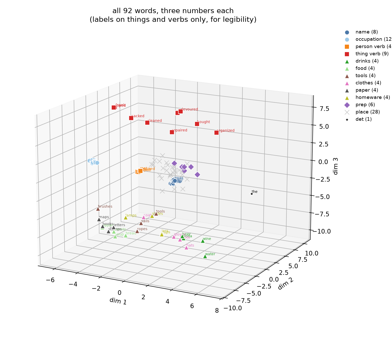
After 3000 small steps of nudging those numbers a little to the left or to the right to make the right next word a bit more likely, here is what the table looks like. All 92 words, three numbers each, plotted as points in space:
The learned embeddings
The three coordinates of all 92 words after training, one colour per kind. Labels are only drawn on things and verbs, for legibility. Nothing told the model which words belong together.
The words sort themselves out by the job they do in a sentence. The nine thing-verbs (red) fly off to the top, far from everything and from each other, because a verb only ever follows a person phrase and never follows an object. The four person-verbs (orange) stay near the middle, next to the names and occupations (blues), which crowd around the centre since those show up in every slot. The 24 things flatten into a disc at the bottom, and inside that disc the drinks sit with the drinks, the tools with the tools, the paper with the paper. Even the article “the” ends up alone, because it is unlike any other thing in our world.
This clustering is not just something the eye wants to see. Running k-means with six clusters over the 24 thing embeddings recovers the true classes 70.8% of the time, against 16.7% for chance. The drinks come back perfect, with “wine”, “water”, “soda” and “beer” in one cluster. Tools and clothes merge into one, which is fair enough, since both get cleaned and packed by the same verbs. The 3-dimensionality of the embeddings just happens to be small enough so that we can draw them in a simple 3D scatterplot. Moving to higher dimensions to improve accuracy destroys this nice property.
Training
But how do we fill in \(\mathbf{W}\) and \(\mathbf{E}\)? The model is initially populated with random values. Training is the part that fills these, and it uses the whole world: all 2560 sentences, every prefix of each one, 11408 next-word questions of the form “john drank” -> water. There is no split and nothing held back. The question here is how much of the world we can fit into those 552 numbers. The model will never generalize to unseen text, as there is no unseen text at all! In a sense, the model is a compressor for our world.
The loop does one thing at a time. Show the model a real prefix and the word that actually came next, compare its 92 percentages with the truth using cross-entropy, ask backpropagation which way to nudge each of the 552 numbers to make the loss smaller, nudge them a little with Adam, repeat. In code that is four lines, because the whole model is one multiplication, another multiplication and a softmax, so the effect of every number on the loss can be worked out exactly and all at once. Nothing is ever written down as a rule. “Drinks follow drank” is not in the code, it is only in the numbers the training ends up choosing.
3000 turns of that take 18 seconds on one CPU core. The first hundred carry almost everything: the loss falls from 6.56, which is guessing, to 2.46 and 26% accuracy. Step 300 has it at 2.04 and 28.6%, and the remaining 2700 steps buy six tenths of a point, ending at 1.99 and 29.2%. From there on the model has taken what a bag of words has to give, and the nudges only reshuffle answers that were already near-tied.
Where the accuracy sits is worth a look, because it points straight at the difficulty. The word “the” is predicted 100% of the time, and rightly so: it is the only word that ever follows a preposition, so when a place phrase starts there is nothing to get wrong. Verbs come out at 14.8% and the things at 9.1%, and those are exactly the slots where several words fit equally well. That is the ceiling again, seen from the other side: the model is not failing at those, the world is ambiguous there. Make it wider, give it 16 numbers per word and a hidden layer, and it climbs from these 29.2% to the ceiling itself, which is what the next section is about.
Results
TinyLM is implemented in PyTorch. The whole experiment, logs and all, is at https://codeberg.org/langurmonkey/tinylm. Every number in this section comes from a run in logs/, all with the same learning rate (0.03), the same 3000 steps and seed 0.
The baseline is the 552-number model from above: 29.2% next-word accuracy, against a ceiling of 48.4%. There are two knobs to turn, so let me turn them one at a time.
More hidden units
First, fix the embeddings at 3 numbers per word and grow the hidden layer from nothing to 128:
| Hidden units | Parameters | Loss | Accuracy |
|---|---|---|---|
| 0 | 552 | 1.991 | 29.2% |
| 2 | 560 | 1.993 | 29.1% |
| 4 | 752 | 1.979 | 29.4% |
| 8 | 1136 | 1.968 | 29.8% |
| 16 | 1904 | 1.948 | 30.7% |
| 32 | 3440 | 1.928 | 31.3% |
| 64 | 6512 | 1.878 | 32.9% |
| 128 | 12656 | 1.826 | 34.9% |
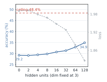
The first thing to notice is how flat the left half is. Going from 0 to 2 hidden units does nothing at all, in fact it loses a tenth of a point, and 4 and 8 buy so little that they are inside the noise. The hidden layer only starts to pay somewhere around 16, and even then the whole sweep, a model 23 times bigger, gets from 29.2% to 34.9%.
That is not the hidden layer’s fault but what (little) it has to work with. There is only a point of three numbers going in, so the yes/no questions the hidden units can ask are questions about three numbers. Everything the model knows about a word is already squeezed into those three numbers before the layer gets a chance to help.
Higher embedding dimensionality
Now fix the hidden layer at 128 and grow the embeddings instead:
| Numbers per word | Parameters | Loss | Accuracy |
|---|---|---|---|
| 3 | 12656 | 1.826 | 34.9% |
| 4 | 12876 | 1.711 | 38.8% |
| 8 | 13756 | 1.476 | 47.4% |
| 16 | 15516 | 1.425 | 48.4% |
| 32 | 19036 | 1.424 | 48.4% |
| 64 | 26076 | 1.424 | 48.4% |
| 92 | 32236 | 1.533 | 44.5% |
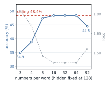
This is a different picture. Four extra coordinates, 220 more numbers, are worth four points, and at 8 numbers per word the model is at 47.4%, basically at the ceiling. At 16 it sits exactly on it, 48.4%, and then nothing happens: 32 and 64 coordinates give the identical number, with the same loss to four decimals. All the extra numbers do is cost time. The model has run out of things to learn, because 48.4% is a property of the world.
Two rows caught my eye: embedding dimensions 16 and 92. At 16 coordinates the positions go to 100%: every preposition that starts a place phrase is now predicted perfectly, whereas at 3 coordinates it was 42.3%. And the last row, 92 coordinates, which is one number per word with no sharing between words, falls back to 44.5%. With a coordinate per word each word is just itself and nothing has to be shared, so the model stops learning that “wine” and “beer” behave alike and learns 92 independent words instead. Fewer is genuinely better here, up to a point.
So the answer to the opening question is 15516 numbers, of which 552 were enough for a quarter of the world and none of them buy anything past the entry at 16. The smallest thing that works is still the 552-number model. The smallest thing that hits the ceiling is the one with 16 coordinates per word.
How well does it compress the world?
Accuracy tells you how often the model is right, but the model is a description of the world, so we can ask the compressor’s question: how many bits does it take to send the whole world using this model? That is the model itself plus the residual, the part the model cannot predict, which the loss measures directly:
- Model cost: parameters \(\times\) 32 bits (unquantized float32, an upper bound).
- Residual: \(N \times loss / ln(2)\) bits, with N = 11408 next-word questions.
- Raw world: \(N \times log_{2}(92)\) ≈ 74421 bits (9.1 KiB), i.e. naming one of 92 words per question with no model at all.
| Model | Params | Bits | Residual | Total | × raw |
|---|---|---|---|---|---|
| 3 coords, no hidden | 552 | 17664 | 32762 | 50426 | 0.68 |
| 3 coords, hidden 128 | 12656 | 404992 | 30051 | 435043 | 5.85 |
| 8 coords, hidden 128 | 13756 | 440192 | 24292 | 464484 | 6.24 |
| 16 coords, hidden 128 | 15516 | 496512 | 23451 | 519963 | 6.99 |
| 92 coords, hidden 128 | 32236 | 1031552 | 25222 | 1056774 | 14.20 |
Only the first row compresses: 0.68× raw. Every row past it spends far more bits on the model than it ever saves on the residual, which bottoms out around 23-24 kbit once the ceiling is reached. I kind of expected this: the smallest thing that compresses is the 552-number baseline, while the smallest thing that predicts at the ceiling is the 15516-number model. Past 16 coordinates even the residual grows again, so the 92-coordinate case is totally hopeless.
Conclusions
TinyLM works because the world is tiny and closed: 92 words, one sentence shape, 11408 questions with nothing held back. To get from here to something GPT-2-like, which predicts arbitrary text, roughly four things have to change, all of them about giving up that closedness.
- The first is obvious: order. The bag of counters has to go, replaced by a sequence with positions and a mechanism that looks at who came before whom: causal self-attention, stacked into a transformer. That alone removes the ceiling.
- The second is also rather self-evident: vocabulary. 92 whole words become ~50k subword pieces (BPE), so the model can spell anything, at the cost of a readout 500 times wider.
- The third is data. Training on everything there is has to become training on gigabytes with text held back, so the score measures generalization instead of memorization.
- Finally, we have scale. One hidden layer becomes 12 layers of 768 numbers (GPT-2 small, 124M parameters), and seconds on a CPU core become hours on a GPU.
Nothing else changes. The objective is still "guess the next word", the loss still means nats, word embeddings are still there, and the compressor’s accounting from the previous section still applies. What changes is only what the model is asked to compress.