Supercharging exoplanets
A short report on the new developments in exoplanet datasets in Gaia Sky
A couple of years ago I wrote about the procedurally generated planets in Gaia Sky. In this post, I provided a more or less detailed technical overview of the process used to procedurally generate planetary surfaces and cloud layers.
Since then, we have used the system to spice up the planets in the planetary systems for which the Gaia satellite could determine reasonable orbits (see the data here, and some Gaia Sky datasets for some of those systems here, including HD81040, Gl876, and more).
However, with the upcoming Gaia DR4, the number of candidate exoplanets is expected to increase significantly, rendering the “one dataset per system” approach unmaintainable. In this post I describe some of the improvements made with regards to exoplanets in Gaia Sky, in both the handling of large numbers of extrasolar systems seamlessly, and in the brand new, improved procedural generation of planetary surfaces and clouds.
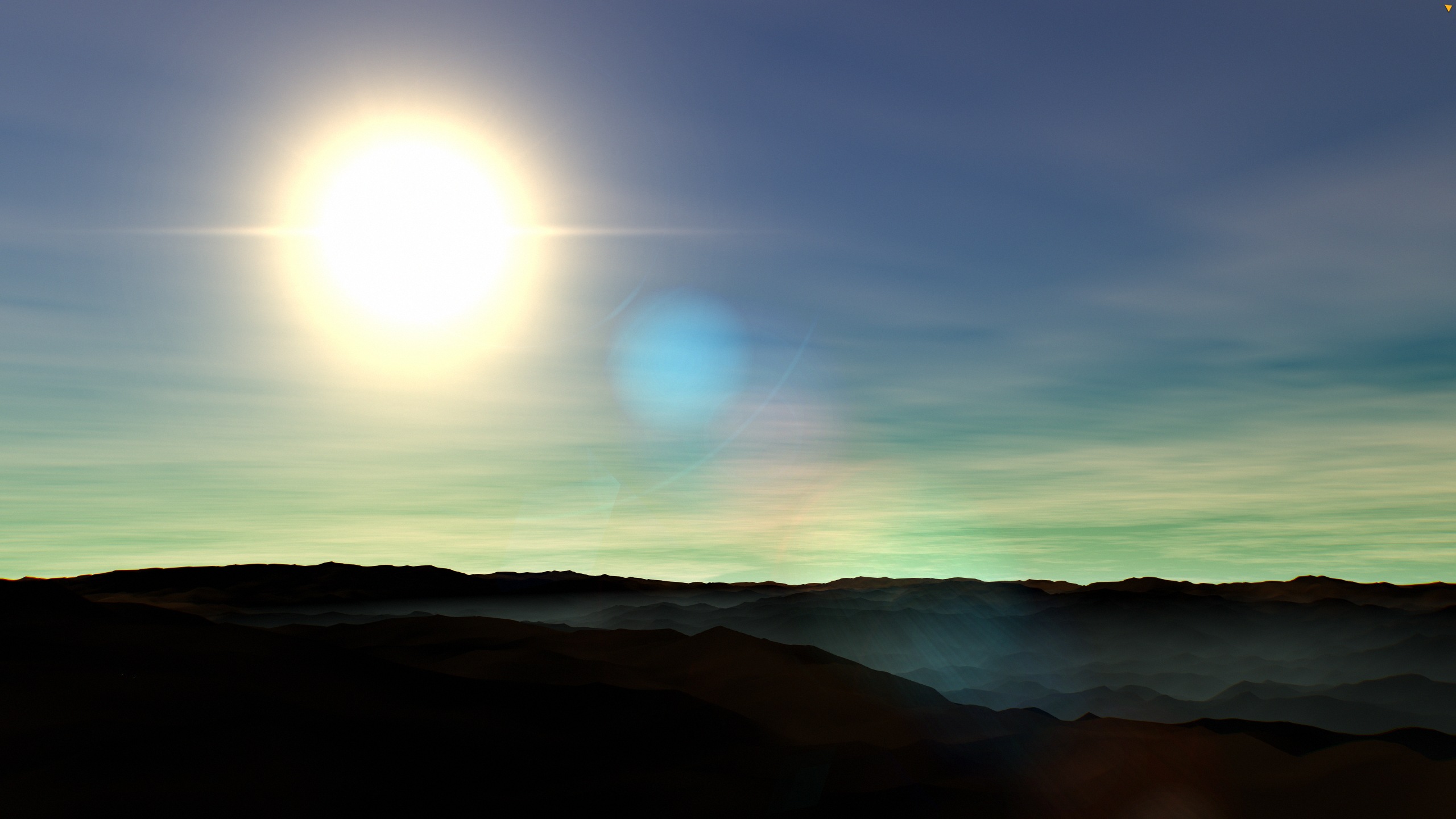
A screenshot from the surface of a procedurally generated planet, in Gaia Sky. In the picture we can see elevation, clouds, atmosphere and fog. This uses the new system.
Representing Exoplanets
So far, Gaia Sky was able to represent extrasolar systems via additional datasets containing the system objects and metadata (barycentre, stars, planets, orbits, etc.). These datasets were and are distributed as standalone downloads via the integrated download manager, which serves data from our data repository. This approach was only good as far as the number of systems was kept low, which was true until now. However, with the advent of DR4, this number is expected to reach four digits, so a new solution is in order.
The representation of exoplanet locations has been in Gaia Sky since 3.6.0, released in March 2024. It is based on the NASA Exoplanet Archive, which contains some 5600 confirmed planets. Up to now, this was implemented as a glorified point cloud, where the glyph for each system is chosen according to the number of candidate planets in said system. Broman et al. developed a more extensive use of glyphs for representing exoplanets in Open Space in ExoplanetExplorer1, and we certainly were inspired by this work.
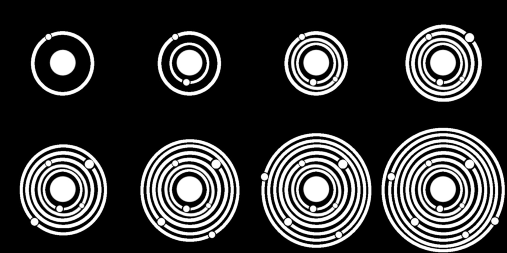
The textures used for exoplanets, sorted from 1 to 8 candidates (1-4 top, 5-8 bottom).
Below is a view of the NASA Exoplanet Archive from the outside. The elongated arm to the left is the Kepler field of view.
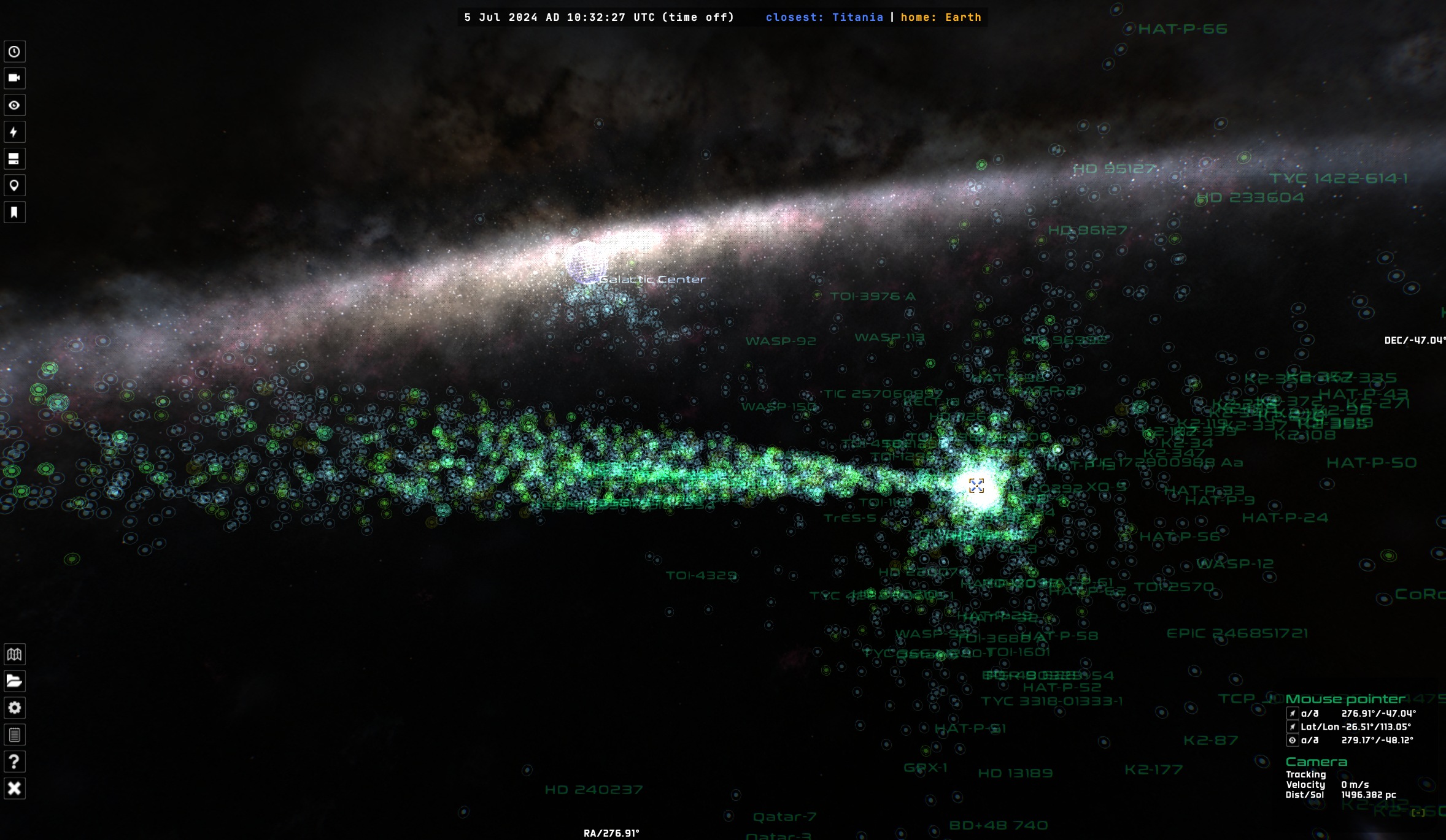
The NASA Exoplanet Archive in Gaia Sky, represented as a point cloud with glyphs.
This representation is useful to indicate the position and number of planets of each system. It works using the particle set object, which is essentially a point cloud. An extension was necessary, in order to select a texture for each system according to the value of one of the table columns. In this case, the texture is selected according to the number of planets in the system. This is done by means of the new textureAttribute attribute in particle sets.
Seamless Fly-In
The first objective in this little project was to achieve a seamless navigation from the “global” view to the “local” view in a seamless way without having to preload all systems’ descriptors at startup. The global view represents the full dataset observed from afar, while the local view represents a rendering of each star system with the exoplanets orbiting around. Additionally, the mechanism used for this should be, if possible, generic for all particle sets.
The base data file is a VOTable as downloaded from the NASA Exoplanet Archive website. This VOTable contains all the available information for each of the planets: name, host name, position, physical characteristics, orbital information, etc.
In order to achieve this seamless navigation, we considered two different options, taking into account that new objects representing the systems need to be loaded at some point:
- Generate the system objects transparently directly in Gaia Sky whenever the camera gets close enough.
- Pre-compute the system descriptor files beforehand and order Gaia Sky to load them whenever the camera nears the object.
Option one has the advantage that the dataset to distribute is much smaller. It only contains the metadata and the VOTable data file. However, this one solution is, by design, very ad-hoc to this dataset in particular. In other words, it would not be easily extensible to other exoplanet datasets (e.g. Gaia DR4) without major code changes.
Option two is much more general, in the sense that it can be applied to all exoplanet catalogs, provided all the Gaia Sky descriptor files are generated. However, the distributed package is a bit heavier, as it needs to include an extra JSON descriptor file for each system. But those are usually small, and compress well.
Proximity Loading
In the end, the positives of the second option vastly outweigh the negatives, so that’s what we went with. We generated the descriptor files with a Python script that aggregates all planets in the same system and produces a series of JSON files. Then, we added a couple of attributes to particle sets:
- “proximityDescriptorsLocation” – the location of the descriptor files for the objects of this particle set. The descriptor files must have the same name as the objects.
- “proximityThreshold” – solid angle, in radians, above which the proximity descriptor loading is triggered.
In principle, any particle set can define these two attributes to enable proximity loading. In it, when the solid angle of a particle overcomes the proximity threshold, the load operation is triggered, where the JSON descriptor file corresponding to the particle gets loaded, if it exists (in the location given by “proximityDescriptorsLocation”). The matching is done using the particle’s name, which must be the same as the file name plus extension.
There are a few requirements for it to work:
- Particles in the particle set must have a name.
- The proximity descriptors location, and optionally the proximity threshold angle, must be defined for the particle set.
- The JSON files to load must be prepared and available at the given location.
The loading itself happens in a background thread. When it is done, the scene graph and the indices are updated. Then, if the camera is in focus mode, and the focus object is the trigger particle, the camera automatically switches focus to the first object in the dataset. Ideally, the first object in the dataset should have the same position as the particle in order to prevent a sudden seeking camera pan.
Proximity loading in Gaia Sky. Each of the extrasolar systems visited in the video gets loaded on-demand when the camera gets close enough to it. Disregard the slow procedural generation in the video, this version is using the old CPU based code. The next chapters in this article contain a description of how we made this much better.
The video above shows the concept of proximity loading in motion. As the camera gets near an object, the proximity loading is triggered and new objects are loaded. When they become available, the camera switches focus to the new object. This results in a seamless exploration from the global dataset to the individual planets of each system.
Procedural Generation Revisited
As mentioned in the beginning, back in 2021 we had a first look at the procedural generation of planetary surfaces. This first approach was based on CPU code that ran rather slowly, so we had to add some progress bars at the bottom of the screen for each of the channels to provide some feedback to the user about the status of the generation. This was less than ideal, so we set up a project to revisit this procedural generation and improve it, if possible.
This project had the following aims:
- Replace the CPU-based code with a GPU implementation that runs much faster.
- Improve the procedural generation to produce higher fidelity, more believable planets.
- Enhance and simplify the procedural generation module and window so that it is easier to use and understand.
GPU Noise and Surface Generation
The first step is straightforward to explain. Essentially, we moved the code from the CPU to the GPU. But the devil is in the details, so let’s dive in.
Previously, we were basing on the Joise library, a pure Java implementation of some common noise functions and layering strategies. From that, we created matrices in the main RAM for the elevation and the moisture, and we filled them up in the CPU using this library. From that, we generated the diffuse, specular and normal bitmaps, created the textures and set up the material. Easy enough.
Now, in the GPU we have two options:
- Pixel shaders.
- Compute shaders.
On the one hand, pixel shaders are ubiquitous and supported everywhere, but they are a bit difficult to use for compute operations, and typically require encoding and decoding information using textures. On the other hand, compute shaders are perfect for this task, as they accept data inputs directly, but they are only in OpenGL since version 4.3. This leaves out, for example, macOS (only supports 4.1) and many systems with older graphics cards.
For the sake of compatibility, we decided to use pixel shaders in favor of compute shaders. They are more difficult to work with, but they should be universally compatible. Moreover, we can embed them directly in a website, like this curl noise, which is pretty neat:
Curl noise shader, with turbulence and ridge, running in the browser.
Code: curl.glsl
But back to the topic, we based our implementation on the gl-Noise library. We fixed some issues and modified it a bit to better suit our need. We ended up implementing fBm for all noise types. fBm is a way to recursively add finer detail to our noise by increasing its frequency and decreasing its amplitude each cycle or octave. The code below shows how to add fBm to any noise function.
#define N_OCTAVES 4

// Initial frequency.
float frequency = 1.0;
// Initial amplitude.
float amplitude = 1.0;

// Frequency increase factor.
float lacunarity = 2.0;
// Amplitude decrease factor.
float persistence = 0.5;

// The noise value.
float val = 0;

// x is the sampling coordinate.
for (int octave = 0; octave < N_OCTAVES; octave++) {
    val += amplitude * noise(frequency * x);
	frequency *= lacunarity;
	amplitude *= persistence;
}
Adding a couple of fBm octaves to the previous Curl noise shader, to get a total of 3 cycles, we get something with much finer detail and more convincing:
Curl noise with 3 octaves.
Code: curl-fbm.glsl
We also changed the noise types from gradval, perlin, simplex, value and white to perlin, simplex, curl, voronoi and white.
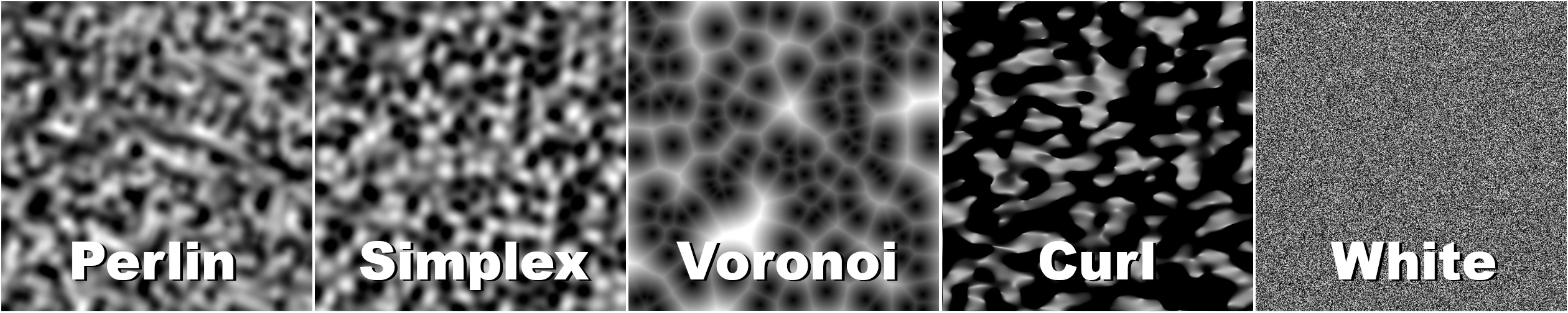
The types of noise supported in the new version.
Since we are creating the noise using shaders, we need to render to an off-screen buffer. We do the process in two passes.
The first pass generates two or three noise channels in a texture. We call it the biome map. The channels are:
- Red: Elevation.
- Green: Moisture.
- Blue (optional): Temperature.
In this pass, we can additionally add another render target to create an emissive map. We’ll cover this later.
The second step uses a frame buffer with multiple render targets, gets the biome map generated in step 1 as input, together with some parameters like the look-up table, and outputs the diffuse, specular, normal and emissive maps. Those are then used to texture the object.
An example using simplex noise is shown below. Note the biome map only has the red and green channels active (for elevation and moisture) in this example.
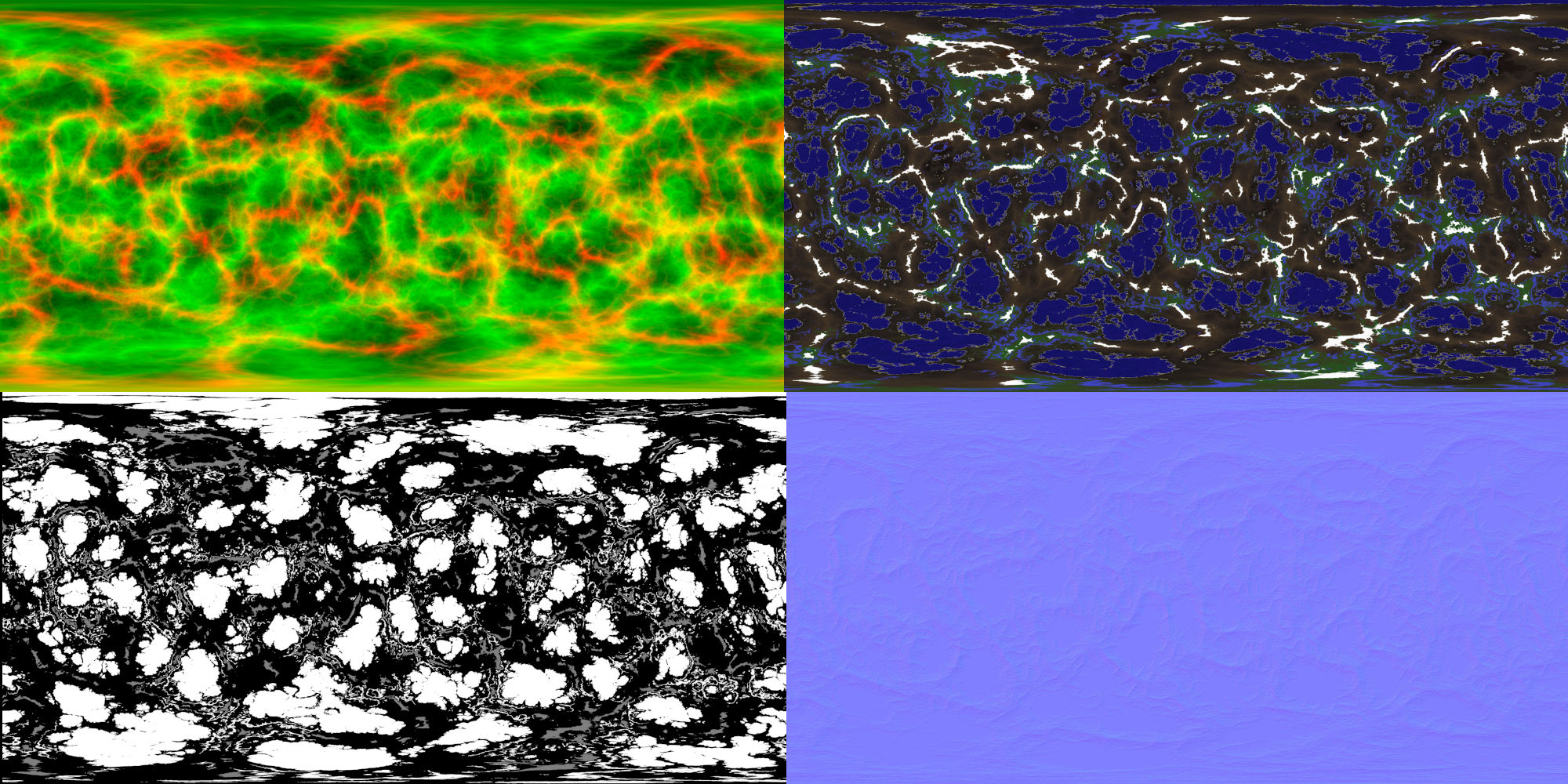
Generated maps for a random planet. From left to right and top to bottom: biome (elevation and moisture) map, diffuse textrue, specular texture and normal texture.
Normal map – Note that the normal texture is only generated if needed, which is when ’elevation representation’ is set to ’none’ in the Gaia Sky settings. If elevation representation is set to either tessellation or vertex displacement, the normals are computed from the orientation of the surface itself, and the normal map is redundant.
Emissive map – Additionally, we may choose to create an emissive map in an additional render target in the biome buffer using a combination of the base noise and white noise. This is used to add ‘civilization’ to planets by means of lights that are visible during the night, on the dark side. When the emissive map is active, the surface generation step (step 2) renders the regions with lights with black and gray colors, simulating cities or artificial structures.
The maps above correspond to the following planet:
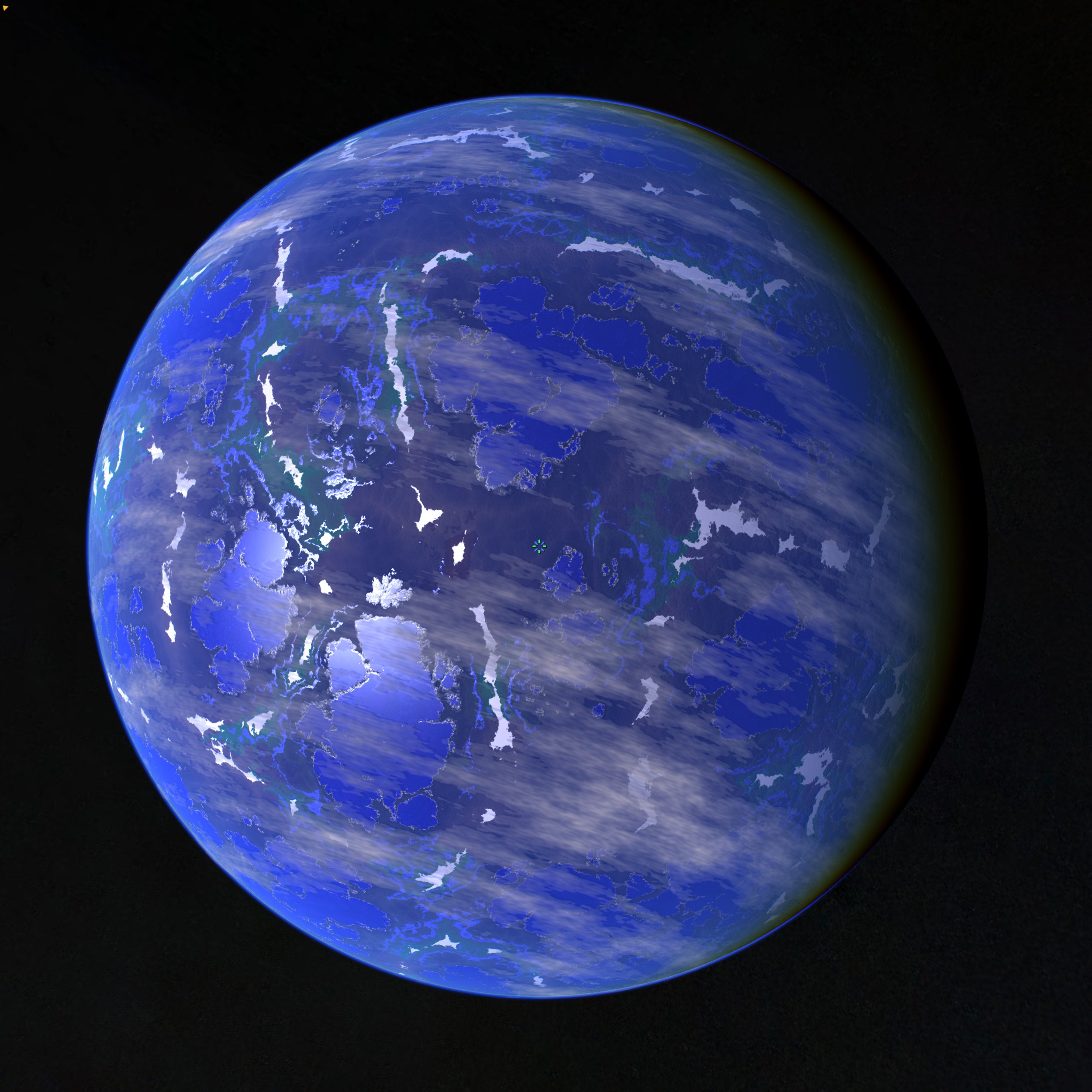
A view of the whole planet corresponding to the maps above. This render also contains a cloud layer, which is generated with the same process and by the same shader as the biome map.
Noise Parametrization
The noise parametrization described in the old post has also changed a bit since then. Essentially, we have now only one fractal type (fBM), the noise types are different, and we have introduced some missing parameters which are important, like the initial amplitude.
- seed – a number which is used as a seed for the noise RNG.
- type – the base noise type. One of perlin2, simplex3, curl4, voronoi5 or white6.
- scale – determines the scale of the sampling volume. The noise is sampled on the 2D surface of a sphere embedded in a 3D volume to make it seamless. The scale stretches each of the dimensions of this sampling volume.
- amplitude – the initial noise amplitude.
- persistence – factor by which the amplitude is reduced in each octave.
- frequency – the initial noise frequency.
- lacunarity – determines how much detail is added or removed at each octave by modifying the frequency.
- octaves – the number of fBm cycles. Each octave reduces the amplitude and increases the frequency of the noise by using the lacunarity parameter.
- number of terraces – the number of terraces (steps) to use in the elevation profile. Set to 0 to not use terraces.
- terrace coarseness – controls the steepness of the terrain in the transition between different terrace levels.
- range – the output of the noise generation stage is in \([0,1]\) and gets map to the range specified in this parameter. Water gets mapped to negative values, so adding a range of \([-1,1]\) will get roughly half of the surface submerged in water.
- power – power function exponent to apply to the output of the range stage.
- turbulence – if active, we use the absolute value of the noise, so that deep valleys are formed.
- ridge – only available when turbulence is active, it inverts the value of the noise, transforming the deep valleys into high mountain ridges.
Presets and UI design
Finally, I want to write a few words about the way the procedural generation UI, which exposes the functionality directly to the user, has changed in Gaia Sky as a result of this migration.
Parameter Presets
First, we have added a series of presets that make it very straightforward to play with the surface generation. These are:
- Earth-like planet.
- Rocky planet.
- Water world.
- Gas giant.
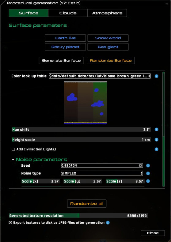
Surface generation tab, wit the preset buttons at the top, in blue.
Each of these is composed of a specific range or value set for each parameter (noise or otherwise), which get automatically applied when the user clicks on the button. So we may have a subset of look-up tables for Earth-like planets, together with a very low initial frequency, and high number of octaves and lacunarity. This is repeated for each of the parameter presets.
Hidden Noise
We have also hidden the noise parameters in a collapsible pane, which produces a cleaner, less cluttered UI.
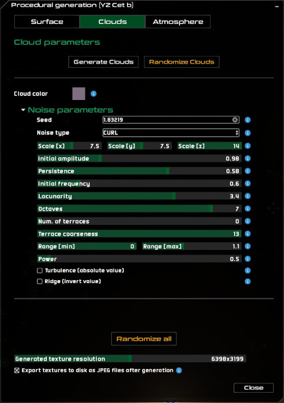
The clouds generation tab shows all noise parameters.
Results
Here are some results produced with the new procedural generation system in Gaia Sky:
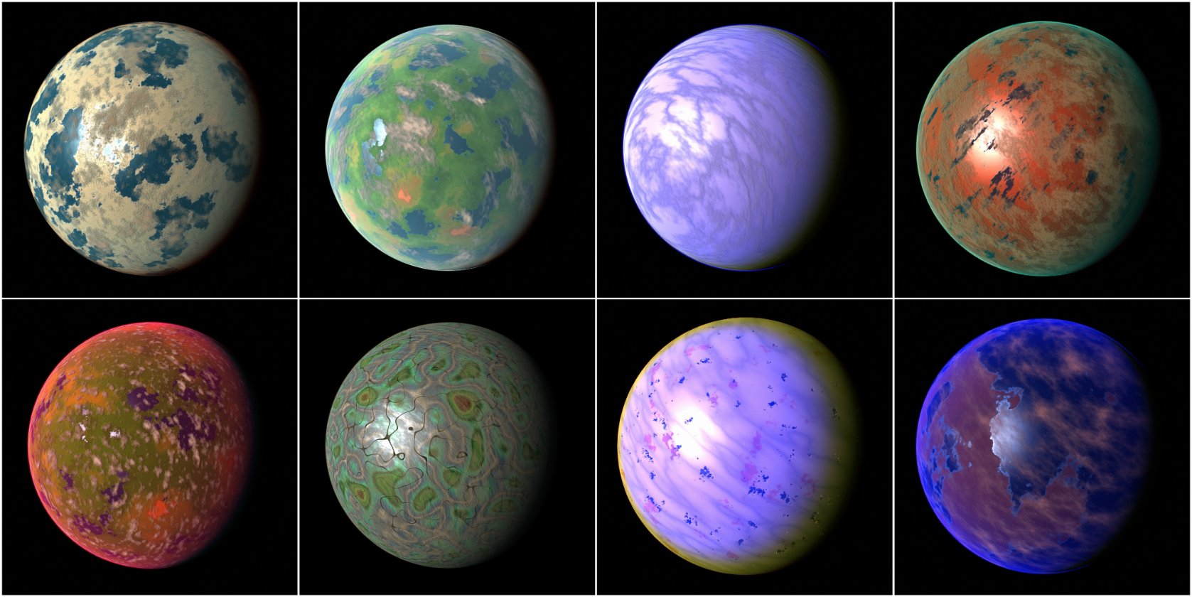
Some procedurally generate planets using the parameter presets, with Gaia Sky.
The improvements described in this post will be released shortly with Gaia Sky 3.6.3 for everyone to enjoy.
E. Broman et al., “ExoplanetExplorer: Contextual Visualization of Exoplanet Systems,” 2023 IEEE Visualization and Visual Analytics (VIS), Melbourne, Australia, 2023, pp. 81-85, doi: 10.1109/VIS54172.2023.00025. ↩︎