Procedural generation of planetary surfaces
Generating realistic planet surfaces and moons
Edit (2024-07-08): We have written a new post to expand on this one. Check it out here.
Edit (2024-06-26): As of Gaia Sky 3.6.3, the procedural generation process has been moved to the GPU. Even though the base method is the same, a number of things have changed from what is described here. For instance:
- The generation is now almost instantaneous, even with high resolutions.
- Gradval and Value noise are no longer available.
- Voronoi and Curl noise are now available.
- The process takes into account a temperature layer.
- We have introduced terraces, with the respective parametrization.
I have recently implemented a procedural generation system for planetary surfaces into Gaia Sky. In this post, I ponder about different methods and techniques for procedurally generating planets that look just right and explain the process behind it in somewhat detail. This is a rather technical post, so be warned. As a teaser, the following image shows a planet generated using the processes described in this article.
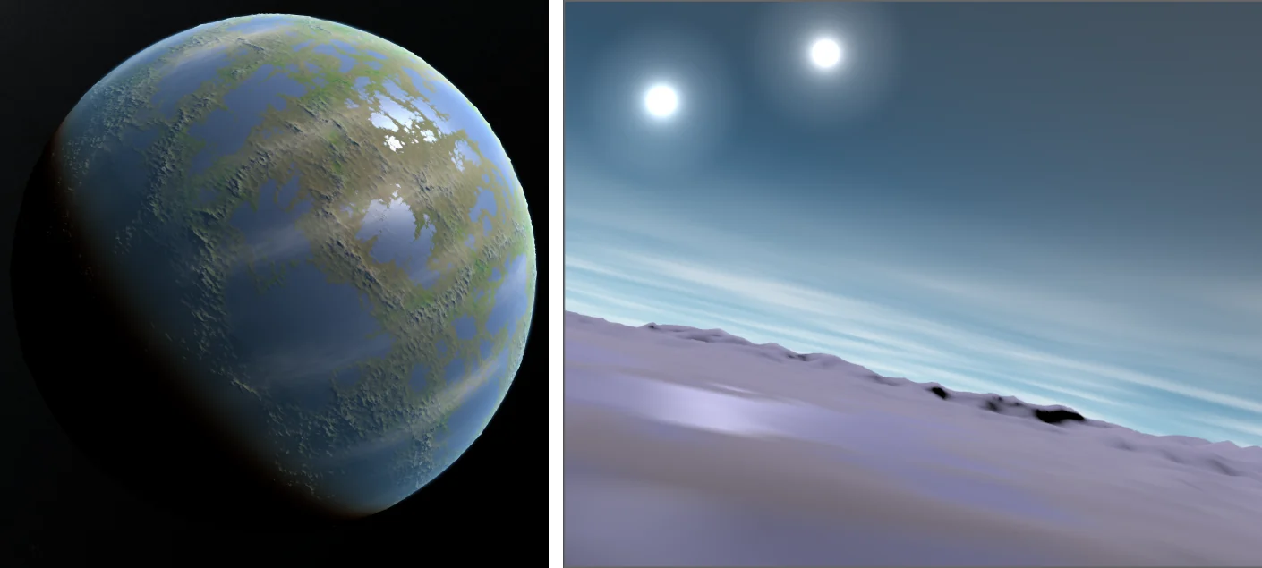
Left: a wide view of a procedurally generated planet. Right: the same planet viewed from the surface.
All is noise
We start with a noise algorithm. A noise algorithm is essentially a function \(f(\vec{x}) = v\) that returns a pseudo-random value \(v\) for each coordinate \(\vec{x}\). The values are not totally random, as they are influenced by where the function is sampled. Obviously, a pure RNG (random number generator) won’t cut it, as the noise we need to generate mountains and valleys and seas is not totally random. There needs to be some structure to it for it to successfully approximate reality. Single values can’t live in isolation, but must depend on their surroundings. In other words, we need smooth gradients. There are very many noise algorithms that are up to the challenge to choose from, but all essentially fall into one of these two categories:
- value noise—based on the interpolation of random values assigned to a lattice of points.
- gradient noise—based on the interpolation of random gradients assigned to a lattice of points.
They are equally valid, but gradient noise is usually more appropriate and visually appealing for procedural generation. One of the most common realization of gradient noise is Perlin noise, developed by Ken Perlin. Let's have a look at some noise generated with this algorithm.
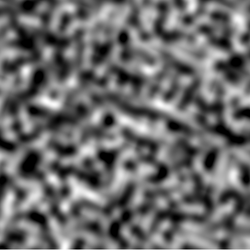
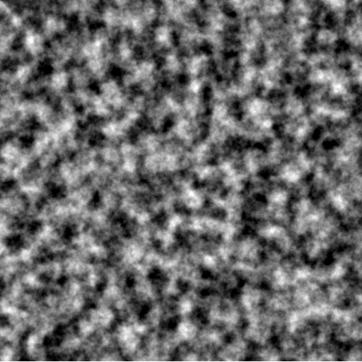
Good old Perlin noise.
It looks alright, but it may not be enough for our purposes as it is now. Let's interpret each pixel in that image as the elevation value at the coordinates of that pixel. This gives us an elevation map. Darker pixels have lower elevations, while brighter pixels have higher elevation. We can then map colors to elevation ranges. Knowing that noise values are in \([0,1]\), we can apply the following mapping:
$$ \begin{align} [0.0, 0.1] &\mapsto blue \\ [0.1, 0.15] &\mapsto yellow \\ [0.15, 0.75] &\mapsto green \\ [0.75, 0.85] &\mapsto gray \\ [0.85, 1.0] &\mapsto white \\ \end{align} $$
Blackish areas are assigned blue, for water. Areas immediately next to water are yellow, for beaches. Gray areas are green, and bright areas are gray and white, for snow. That gives us the following image:
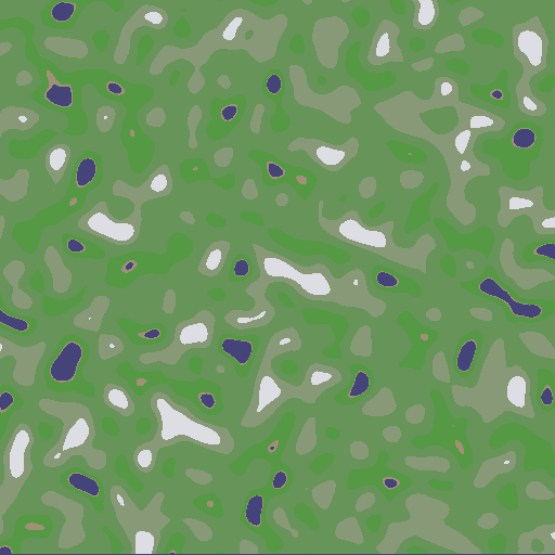
Perlin noise colored with a simple mapping.
Again, it is alright, but it is not super good. It looks plain and not very natural. We can try with other noise algorithms.

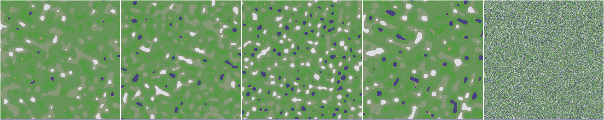
Above: different noise algorithms sampled in the same region. Below: the same noise types colored with the same mapping explained above.
Simplex noise is an evolution of Perlin noise with fewer artifacts. Its open implementation is multi-dimensional and it is also quite fast. The others are also good if used properly.
We can also generate the normal maps from the elevation data. Doing so involves computing the horizontal and vertical gradients for every coordinate. The normal map encodes the direction of the surface normal vector at each point, and works a little better at visualizing the gradients. Additionally, it will come in handy for the shading.
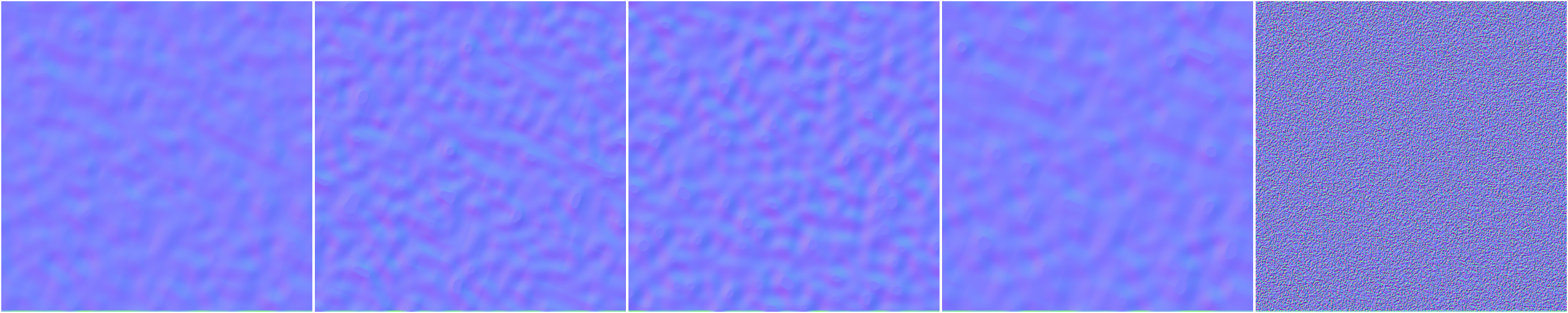
Normal maps generated for the same noise types. Left to right: gradval, perlin, simplex, value, white.
At this point, we need something else. The noise looks too simple and plain. In nature, we have repeating features at different scales, but here we don't see this. These repeating features are called fractals, and we can also create them with the noise algorithms that we already know. The trick is re-sampling the noise function several times with higher frequencies and lower amplitudes. In the context of noise, the different levels are called octaves. The first octave is the regular noise map we have already seen. The second octave would be computed by multiplying the frequency of the first one by a number (called lacunarity) and multiplying its amplitude by another number (called persistence), typically a fraction of one. The third would apply the same principle to the parameters of the second, and so on.
const int N_OCTAVES = 5;
// Initial values
float frequency = 2.5;
float amplitude = 0.5;
// Parameters
float lacunarity = 2.0;
float persistence = 0.5;

// The noise value
float n = 0;

// x and y are the current coordinates
for (int octave = 0; octave < N_OCTAVES; octave++) {
    n += amplitude * noise(frequency * x, frequency * y);
	frequency *= lacunarity;
	amplitude *= persistence;
}
If we run this code with simplex noise, we get the following.
 Open Simplex noise with 4 octaves. | 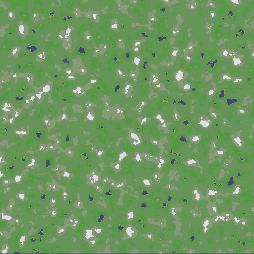 Same noise colored with same process. |
If you zoom in into the left image, you will see that there are additional levels of detail at smaller scales compared to the regular simplex noise shown before. This is very good, as it mimics nature much more closely. We are now ready to start generating surfaces.
Surface generation
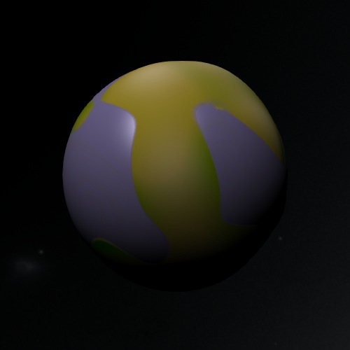
From now on we’ll interpret the generated noise as the terrain elevation and map it to a sphere. For instance, the noise types we saw before look as follows when mapped to a sphere.
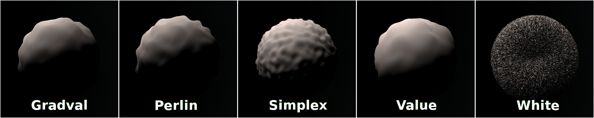
Noise interpreted as elevation and mapped to a sphere.
They all are reasonable, except white. We’ll proceed with simplex from now on.
Colors
In the previous sections we have only mapped colors to elevation ranges, but this produces very little variety. We can generate an additional noise map with the same parameters and interpret it as humidity data, that we can combine with the elevation to produce a color. The elevation data is a 2D array containing the elevation value in \([0,1]\) at each coordinate. The humidity data is the same but it contains the humidity value. We use the humidity, then, together with the elevation, to determine the color using a look-up table. This allows us to color different regions at the same elevation differently. We map the humidity value to the \(x\) coordinate and the elevation to \(y\). Both coordinates are normalized to \([0,1]\).
Additionally, since the look-up table is just an image in disk, we can have many of them and use them in different situations, or even randomize which one is picked up. A simple, discrete look-up table would look like this. From left to right it maps less humidity (hence the yellows, to create deserts, and grays at the top, for rocky mountains) to more humidity (as we go right it gets greener, and the mountain tops get white snow).
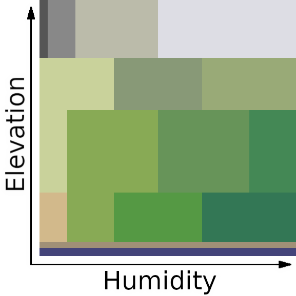
The look-up table mapping dimensions are elevation and humidity.
If we use this look-up table with the simplex noise ball above, we get the following.
Coloring the ball with the discrete look-up table above.
In this image, the noise is mapped to \([0,1]\). We can try extending it to negative values to add some water, as water is mapped to negatives. If we use \([-1,1]\), we get the following.
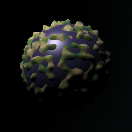
Mapping the noise to [-1, 1].
That is better. But the noise is too high frequency. We can lower it a lot to get larger land masses. We’ll use the higher octaves to add extra details. For now, let’s lower the frequency a lot.
Lowering the frequency produces larger land masses, akin to continents.
Now it is time to smooth things out. We said we can use any look-up table, so how about using one with smooth gradients:

Smooth version of the biome look-up table.
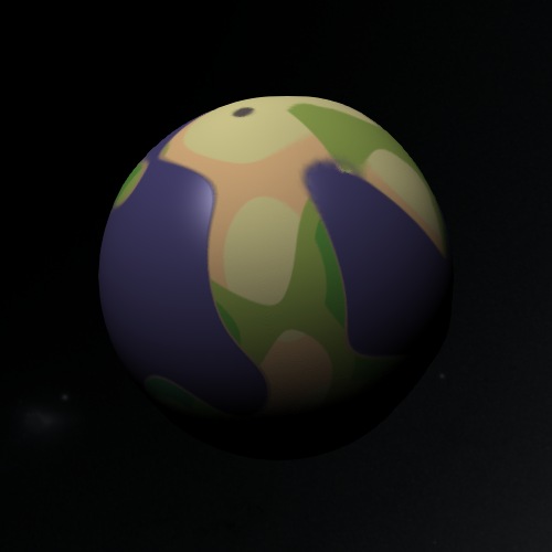
And let’s apply it to the last planet with the low frequency.
The smooth look-up table produces better-looking planets.
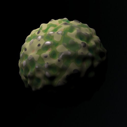
Finally, we can enable additional octaves to produce detail at smaller scales. This step is crucial and is what really sells it. Have a look at this:
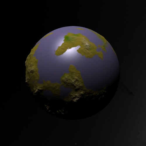
Same planet, but this time around using 8 octaves.
Looks fine, right? In Gaia Sky we can add an atmosphere (computes atmospheric scattering of light in a shader) and add a cloud layer to have this final look.
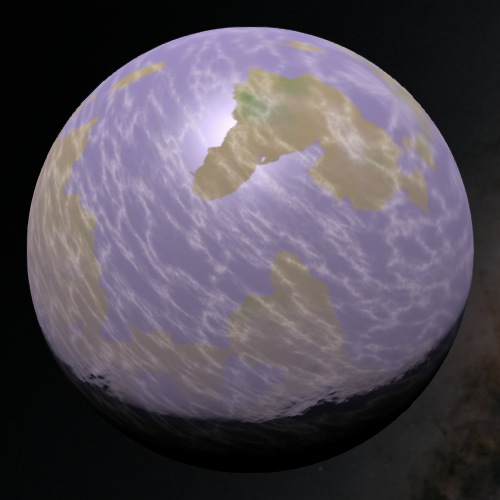
Adding an atmosphere and clouds improves the final result.
Adding some variety
There are some tricks we can use to add some variety to the process.
For example, we can hue-shift the look-up table by a value (in \([0^{\circ}, 360^{\circ}]\)) in order to produce additional colors. The shift must happen in the HSL color space, so we convert from RGB to HSL, modify the H (hue) value, and convert it back to RGB. Once the shift is established, we generate the diffuse texture by sampling the look-up table and shifting the hue.
We can also generate a specular texture where there is water. The specular texture is generated by assigning all heights less or equal to zero to a full specular value. All the planets we have seen so far already apply this specular data.
Seamless (tilable) noise
In this article we have used a little trick that we have not yet talked about. Usually, noise sampled directly is not tileable, but the images in this article do not have seams. If sampled with \(x\) and \(y\) directly, the features do not repeat. In the case of one dimension, usually one would sample the noise using a coordinate for the only dimension available, \(x\).

Sampling noise in 1D leads to seams.
However, if we go one dimension higher, 2D, and sample the noise along a circumference embedded in this two-dimensional space, we get seamless, tileable noise.
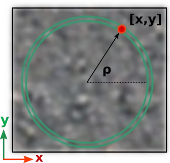
Sampling noise along a circumference in 2D space is seamless
We can apply this same principle with any dimension \(d\) by sampling in \(d+1\). Since we need to create spherical 2D maps (our aim is to produce textures to apply to UV spheres), we do not sample the noise algorithm with the \(x\) and \(y\) coordinates of the pixel in image space. That would produce higher frequencies at the poles and lower around the equator. Additionally, the noise would contain seams, as it does not tile by default. Instead, we sample the 2D surface of a sphere of radius 1 embedded in a 3D volume, so we sample 3D noise. To do so, we iterate over the spherical coordinates \(\varphi\) and \(\theta\), and transform them to cartesian coordinates to sample the noise:
$$ \begin{align} x &= \cos \varphi \sin \theta \nonumber \\ y &= \sin \varphi \sin \theta \nonumber \\ z &= \cos \varphi \nonumber \end{align} $$
The process is outlined in this code snippet. If the final map resolution is \(N \times M\), we use N \(\theta\) steps and M \(\varphi\) steps.
// Map is NxM
for (float phi = -PI / 2; phi < PI / 2; phi += PI / M){
    for (float theta = 0; theta < 2 * PI; theta += 2 * PI / N) {
        n = noise(cos(phi) * cos(theta), // x
                  cos(phi) * sin(theta), // y
                  sin(phi));             // z
        theta += 2 * PI / N;
    }
}
Noise parametrization
We carry out the generation by sampling configurable noise algorithms (Perlin, Open Simplex, etc.) at different levels of detail, or octaves. In Gaia Sky, we have some important noise parameters to adjust:
- seed – a number which is used as a seed for the noise RNG.
- type – the base noise type. Can be any algorithm, like gradient (Perlin) noise1, simplex2, value3, gradval noise4 or white5. For examples, see here.
- fractal type – the algorithm used to modify the noise in each octave. It determines the persistence (how the amplitude is modified) as well as the gain and the offset. Can be billow, deCarpenterSwiss, fractal brownian motion (FBM), hybrid multi, multi or ridge multi. For examples, see here.
- scale – determines the scale of the sampling volume. The noise is sampled on the 2D surface of a sphere embedded in a 3D volume to make it seamless. The scale stretches each of the dimensions of this sampling volume.
- octaves – the number of levels of detail. Each octave reduces the amplitude and increases the frequency of the noise by using the lacunarity parameter.
- frequency – the initial frequency of the first octave. Determines how much detail the noise has.
- lacunarity – determines how much detail is added or removed at each octave by modifying the frequency.
- range – the output of the noise generation stage is in \([0,1]\) and gets map to the range specified in this parameter. Water gets mapped to negative values, so adding a range of \([-1,1]\) will get roughly half of the surface submerged in water.
- power – power function exponent to apply to the output of the range stage.
The final stage of the procedural noise generation clamps the output to \([0,1]\) again, so that all negative values are mapped to 0, and all values greater than 1 are clamped to 1. This means that water is mapped to 0 instead of negative values, but that doesn't change anything.
Finally, we can also generate a normal map from the height map by determining elevation gradients in both \(x\) and \(y\). We use the normal map only when tessellation is unavailable or disabled. Otherwise it is not generated at all. The generation of the normal map is out of the scope of this article.
Cloud layer generation
We can generate the clouds with the same algorithm and the same parameters as the surface elevation. Then, we can use an additional color parameter to color them. For the clouds to look better one can set a larger \(z\) scale value compared to \(x\) and \(y\), so that the clouds are stretched in the directions perpendicular to the rotation axis of the planet.
Putting it all together
In this article we have showed a bird’s eye view of how to procedurally generate convincing planetary surfaces. As we said, in Gaia Sky we generate spherical maps which are then mapped to UV spheres, but we could as well produce cubemap faces and use cubemaps to do the texturing. Below you can see an example of maps produced for a planet by Gaia Sky.
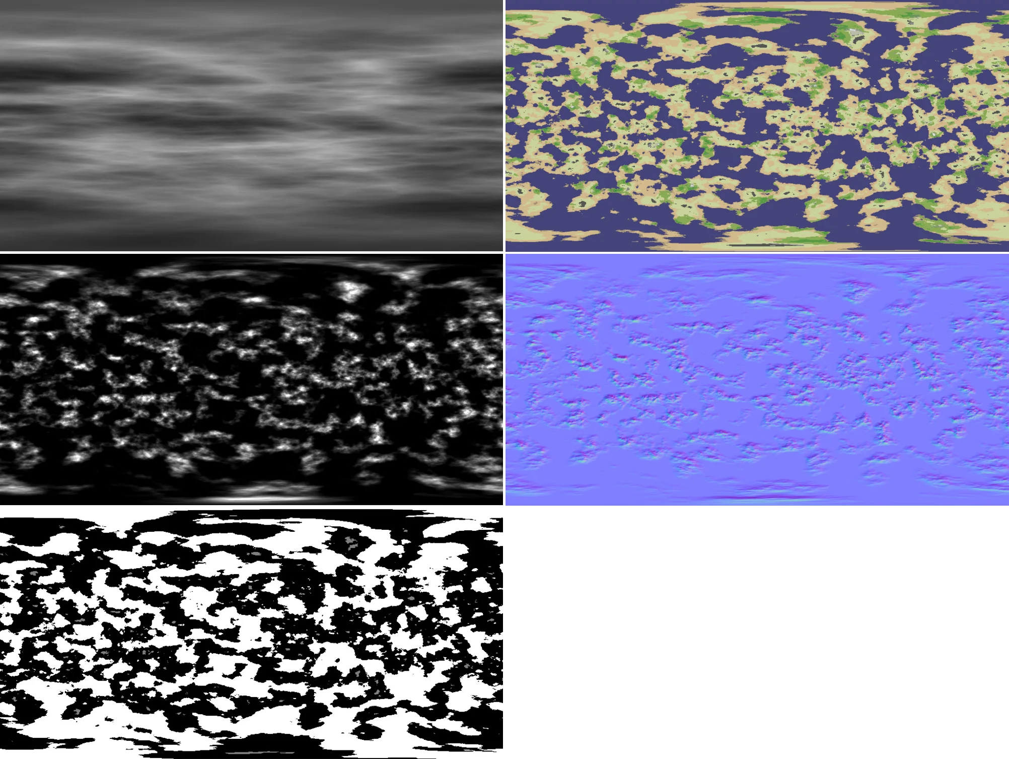
Left to right and top to bottom, clouds map, diffuse texture, elevation map, normal map and specular map procedurally generated with Gaia Sky.
Additionally, we have added a separate step to generate a cloud layer, and we can also randomize the atmospheric scattering parameters to have a fully procedural planet. We have implemented a function which randomizes all parameters within some bounds. Hitting the Randomize all button produces some neat results:
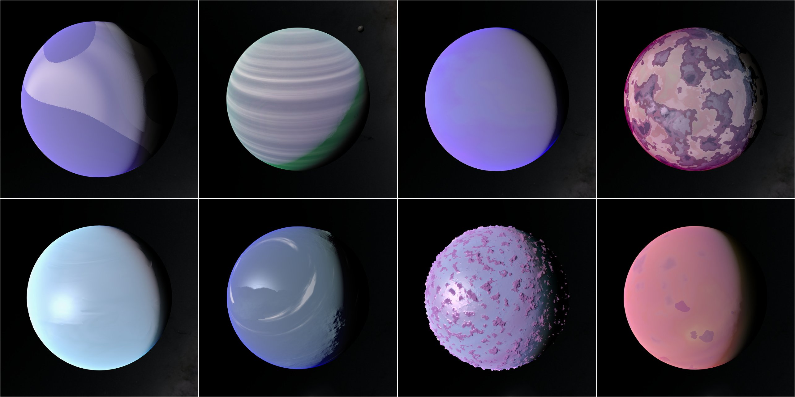
Random planets created with Gaia Sky.
More information on the topic can be found in the official documentation of Gaia Sky.
A hybrid consisting of the sum of gradient and value noise. ↩︎